Example (1D)
Jump to navigation
Jump to search
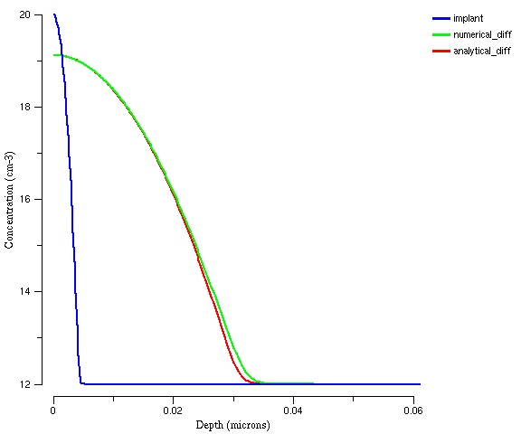
This is an example that uses the "diffuse" command to predict diffusion of an implant profile. The numerical solution is compared to an analytical solution.
Establish diffusion parameters and solution variable "Test"
math diffuse dim=1 umf none col !scale
solution add name=Test solve !negative
pdbSetDouble Silicon Test Abs.Error 1.0e-8
pdbSetDouble Silicon Test Rel.Error 1.0e-2
Establish the grid and assign a material
line x loc=0.0 spac=0.0002 tag=Top
line x loc=0.2 spac=0.001 tag=Bottom
region silicon xlo=Top xhi=Bottom
init
Gaussian implant profile
#fill in file name for as-implanted profile here
sel z=1.0e20*exp(-(x/0.001)*(x/0.001))+1.0e12 name=Test
#plot the the as-implanted profile
sel z=log10(Test)
plot.1d max=0.06 min=[list 0.0 12.0] label=implant
#value for diffusivity goes here
term name = TestDiff add silicon eqn = "4.0e-17"
#solid-solubility limit stuff
term name = TestActive add silicon eqn = "(Test>1.0e20)?1.0e20:Test"
Establish the physics
#simple Fick's law based diffusion equation
pdbSetString Silicon Test Equation "ddt(Test) - TestDiff * grad(TestActive)"
Use "difuse" command to solve
diffuse time = 60.0 temp=550 init=1.0e-1
#plot the the final profile
sel z=log10(Test)
plot.1d !cle max=0.06 min=0.0 label=numerical_diff
Use the "FindDose" command to intigrate the total implant dose and save as "dose"
sel z=Test
set dose [FindDose]
#analytical model for drive-in diffusion
sel z = ($dose*1.0e4)/(sqrt(3.14*4.0e-17*1.0e8*60.0*60.0))*exp(-(x*x)/(4*4.0e-17*1.0e8*60.0*60.0))+1.0e12 name=model
sel z=log10(model)
plot.1d !cle max=0.06 min=0.0 label=analytical_diff
The final plot is shown below. The numerical method slightly over-predicts the diffusion distance.
