Plot Examples: Difference between revisions
No edit summary |
|||
| Line 5: | Line 5: | ||
Grid2D | Grid2D | ||
sel z=1.0e17 name=Boron store | |||
sel z=1.0e15 name=Arsenic store | sel z=1.0e15 name=Arsenic store | ||
implant arsenic dose=1.0e15 energy=20 | |||
strip photo=az | |||
diffuse time=5 temp=1100 dry | |||
<br /> The plot is created with:<br /> | <br /> The plot is created with:<br /> | ||
plot.2d bound fill | |||
sel z = Boron-Arsenic | |||
contour val = 0.0 | |||
sel z = log10(abs(Boron-Arsenic)) | |||
for {set i 15} {$i | for {set i 15} {$i <= 20.0} {incr i} { | ||
contour val = $i | |||
} | } | ||
This code section will draw the | This code section will draw the outline of the device and stretch it to fill the plot window. The next line [select.html selects] the doping concentration and plots a line along the metallurgical junction. Then plot variable is selected to the log base 10 of the absolute doping concentration. A loop from 15 to 20 follows with [contour.html contour] lines being drawn each decade for both p- and n-type doping. The resulting plot: | ||
[[Image:cc.gif]] | [[Image:cc.gif]] | ||
| Line 30: | Line 30: | ||
sel z=log10(Boron) | |||
plot.1d y=-2.0 | |||
sel z=log10(Arsenic) | |||
plot.1d y=-2.0 !cle | |||
This code section will draw the boron and arsenic concentrations at the left edge of the device. Both lines are on the same plot: [[Image:onedblt.gif]] | This code section will draw the boron and arsenic concentrations at the left edge of the device. Both lines are on the same plot: [[Image:onedblt.gif]] | ||
Revision as of 20:40, 6 April 2011
Contour and Color Plots
A structure is created with the following set of commands:
Grid2D
sel z=1.0e17 name=Boron store
sel z=1.0e15 name=Arsenic store
implant arsenic dose=1.0e15 energy=20
strip photo=az
diffuse time=5 temp=1100 dry
The plot is created with:
plot.2d bound fill
sel z = Boron-Arsenic
contour val = 0.0
sel z = log10(abs(Boron-Arsenic))
for {set i 15} {$i <= 20.0} {incr i} {
    contour val = $i
}
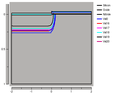
This code section will draw the outline of the device and stretch it to fill the plot window. The next line [select.html selects] the doping concentration and plots a line along the metallurgical junction. Then plot variable is selected to the log base 10 of the absolute doping concentration. A loop from 15 to 20 follows with [contour.html contour] lines being drawn each decade for both p- and n-type doping. The resulting plot:
One-Dimensional Plots
Using the same structure as before, we can perform depth plots through several regions of the device.
sel z=log10(Boron)
plot.1d y=-2.0
sel z=log10(Arsenic)
plot.1d y=-2.0 !cle
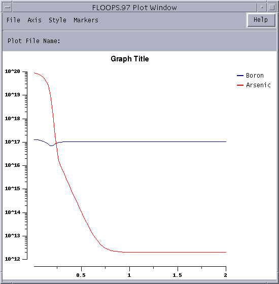
This code section will draw the boron and arsenic concentrations at the left edge of the device. Both lines are on the same plot: 
