Select Examples

Selection Examples

Select Command Examples

select z = log10(Boron)

Select the log10 of the chemical boron concentration.

select z = log10(BoronActive)

Select the log10 of the active boron concentration.

select z = 1.0e18*exp(-x*x/0.0001) store name=Boron

Select a Gaussian profile in x. The value will be used to initialize the field Boron, and the field will be written out when structure files are saved.

TCL Return Functions

Junction Depth and Layers

Grid1D
[select.html sel] z = {1.0e18*exp(-x * x / 0.01) - 1.0e15}
[layers.html layers
]

The above deck initializes the grid with a default one dimensional structure. The second command selects as the plot variable a Gaussian profile minus a background doping. The layers command integrates the selected variable and reports zero crossings. The output is:

	Top          Bottom        Integral    Material
0.00000e 00     2.62905e-01     8.83423e 12    Silicon
0.262905e-1     5.00000e 01    -4.97191e 12    Silicon

The top layer has positive sign and is silicon. The total integrated dose is 8.8e12 in this layer. From 0.26um down, the selected variable is negative. To a depth of 50um, the integrated value is about 5e12.

puts "The Junction Depth is [[interp.html interpolate] silicon z=0.0]"

The above command uses the interpolate command to locate the zero crossing and report the value. For the structure above, the output is:

The Junction Depth is 2.629046e-01

Additional processing can be performed using the [print.1d.html print.1d] command.

set dep 0
foreach f [print.1d] {
    set x [lindex $f 0]

    set y [lindex $f 1]
    if {$y > 0.0} {incr dep}
}
puts $dep

Returns 227, the number of grid points that have a positive selected variable value. Other operations can be performed and are limited only by the tcl capabilities.

Interface Manipulations

Grid1D
[../floops/diffuse.html diffuse] time=60 temp=1100 wet

The above two commands grow an oxide that will be used in the remaining examples.

set top [[interface.html interface] oxide /gas]
set bot [[interface.html interface] oxide /silicon]

puts "Thickness is [expr $bot - $top]"

The interface commands return the location of the interface. Since we can independently locate both the top and bottom, these can be subtracted to obtain the total oxide thickness. The total oxide thickness is 0.673907.

tclsel z = {$Oxidant}
layers

These two commands sel the oxidant and then integrate it across all material layers. The output is:

	 Top          Bottom        Integral    Material
-3.68495e-01     3.05413e-01     1.12857e 15    Oxide
 3.05413e-01     5.00000e 01     2.67928e 12    Silicon

The oxide layer thickness is 0.674, and the dose of oxidant contained in the layer is 1.1e15. The silicon has been consumed as expected.

BLT Plot Window Examples

Contour and Color Plots

A structure is created with the following set of commands:

Grid2D
[select.html sel] z=1.0e17 name=Boron store

[../floops/implant.htm implant] arsenic dose=1.0e15 energy=20
[../floops/strip.html strip] photo=az
[../floops/diffuse.html diffuse] time=5 temp=1100 dry
set Win BLTplot.html#CreateGraphWindow CreateGraphWindow

The variable Win now contains the contact information for the plot window. The window will look like:

The next set of commands adds the material boundaries.

foreach m mater.html mater {
    [BLTplot.html#CreateBound CreateBound] $Win $m [[bound.html bound] $m]
}
[BLTplot.html#FlipY FlipY] $Win 1

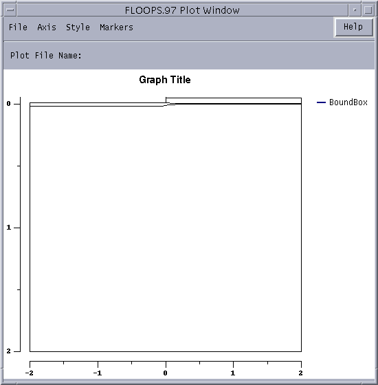
The abouve section of commands duplicates the old style "plot.2d bound" command. The plot window looks:

.

[select.html sel] z = { Boron-Arsenic }
[BLTplot.html#CreateLine CreateLine] $Win Junction [[slice.html slice] silicon val = 0.0]

These two commands select the net doping and then plot a contour line along the material junction.

[select.html sel] z = { log10(abs( Boron-Arsenic) ) }
for {set i 18} {$i <= 20.0} {incr i} {
    [BLTplot.html#CreateLine CreateLine] $Win $i [[slice.html slice] silicon val = $i]

}

This set puts isoconcentration lines on the plot. After [BLTWindow.html changing] the line style for the various elements, and selecting fill for the oxide and nitride. These options are selected in the [BLTWindow.html BLT plot window]. The final graph looks like :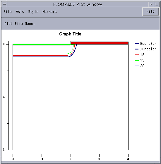

One-Dimensional Plots

Using the same structure as before, we can perform depth plots through several regions of the device.

[BLTplot.html#ClearGraph ClearGraph] $Win
[select.html sel] z=Boron
[BLTplot.html#CreateLine CreateLine] $Win Boron [[slice.html slice] silicon y = -2.0]
[select.html sel] z=Arsenic
[BLTplot.html#CreateLine CreateLine] $Win Arsenic [[slice.html slice] silicon y = -2.0]

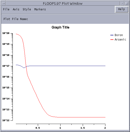
This code section will draw the boron and arsenic concentrations at the left edge of the device. Both lines are on the same plot.

Grid Plot

We create a structure with an interesting grid using the commands:

Grid2D
foreach m [mater] {Smooth $m}

This smooths each region of the mesh.

foreach m mater.html mater {
    [BLTplot.html#CreateBound CreateBound] $Win $m [[bound.html bound] $m]
}
FlipY $Win 1

This code section outlines each section. The grid can be plotted using a combination of the element command and the CreateLine command.

foreach m mater.html mater {
    [BLTplot.html#CreateLine CreateLine] $Win $m [[element.html element] $m]
}

Each material has its grid added to the plot. After some [BLTWindow.html property editing], the plot looks like: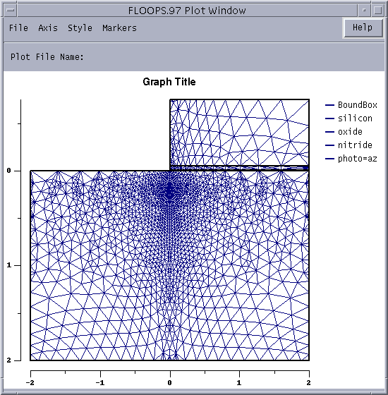

XGraph Window Examples

Contour and Color Plots

A structure is created with the following set of commands:

Grid2D
[select.html sel] z=1.0e17 name=Boron store
sel z=1.0e15 name=Arsenic store
[../floops/implant.htm implant] arsenic dose=1.0e15 energy=20
[../floops/strip.html strip] photo=az
[../floops/diffuse.html diffuse] time=5 temp=1100 dry

The plot is created with:

[plot.2d.html plot.2d] bound fill
[select.html sel] z = Boron-Arsenic
[contour.html contour] val = 0.0
[select.html sel] z = log10(abs(Boron-Arsenic))
for {set i 15} {$i <= 20.0} {incr i} {
    [contour.html contour] val = $i
}

This code section will draw the [plot.2d.html outline] of the device and stretch it to fill the plot window. The next line [select.html selects] the doping concentration and [contour.html plot]s a line along the metallurgical junction. Then plot variable is selected to the log base 10 of the absolute doping concentration. A loop from 15 to 20 follows with [contour.html contour] lines being drawn each decade for both p- and n-type doping. The resulting plot: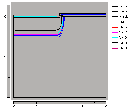

One-Dimensional Plots

Using the same structure as before, we can perform depth plots through several regions of the device.

[select.html sel] z=log10(Boron)
[plot.1d.html plot.1d] y=-2.0
[select.html sel] z=log10(Arsenic)
[plot.1d.html plot.1d] y=-2.0 !cle

This code section will draw the boron and arsenic concentrations at the left edge of the device. Both lines are on the same plot: