|
|
| (5 intermediate revisions by 2 users not shown) |
| Line 1: |
Line 1: |
| === Contour and Color Plots ===
| | = Contour and Color Plots = |
|
| |
|
| A structure is created with the following set of commands: | | A structure is created with the following set of commands: |
| Line 5: |
Line 5: |
| | | |
| Grid2D | | Grid2D |
| [pselectCommandl sel]] z=1.0e17 name=Boron store | | sel z=1.0e17 name=Boron store |
| [[implantCommand | implant]] arsenic dose=1.0e15 energy=20
| |
| [[stripCommand | strip]] photo=az
| |
| [[diffuseCommand | diffuse]] time=5 temp=1100 dry
| |
| set Win[ [[CreateGraphWindow]]]
| |
| | |
| The variable Win now contains the contact information for the plot window. The window will look like:
| |
| | |
| [[Image:Blank.gif]]
| |
| | |
| The next set of commands adds the material boundaries.
| |
| | |
|
| |
| foreach m [[materCommand | mater]] {
| |
| [[CreateBound]] $Win $m [ [[bound]] $m]
| |
| }
| |
| [[BLTplot | Flipy]] $Win 1
| |
| | |
| The abouve section of commands duplicates the old style "plot.2d bound" command. The plot window looks:
| |
| | |
| [[Image:bound.gif]].
| |
| | |
|
| |
| [[selCommand | sel]] z = { Boron-Arsenic }
| |
| [[BLTplot | CreateLine]] $Win Junction [ [[sliceCommand | slice]] silicon val = 0.0]
| |
| | |
| These two commands select the net doping and then plot a contour line along the material junction.
| |
| | |
| [[selectCommand | sel]] z = { log10(abs( Boron-Arsenic) ) }
| |
| for {set i 18} {$i <= 20.0} {incr i} {
| |
| [[BLTplot | CreateLine]] $Win $i [ [[sliceCommand | slice]] silicon val = $i]
| |
| }
| |
| | |
| | |
| This set puts isoconcentration lines on the plot. After [[BLTWindow | changing]] the line style for the various elements, and selecting fill for the oxide and nitride. These options are selected in the [[BLTWindow | BLT plot window]]. The final graph looks like :
| |
| | |
| [[Image:ccblt.gif]]
| |
| | |
| === One-Dimensional Plots ===
| |
| | |
| Using the same structure as before, we can perform depth plots through several regions of the device.
| |
| | |
|
| |
| [[BLTplot | ClearGraph]] $Win
| |
| [[selCommand | sel]] z=Boron
| |
| [[BLTplot | CreateLine]] $Win Boron [ [[sliceCommand | slice]] silicon y = -2.0]
| |
| [[selCommand | sel]] z=Arsenic
| |
| [[BLTplot | CreateLine]] $Win Arsenic [ [[sliceCommand | slice]] silicon y = -2.0]
| |
| | |
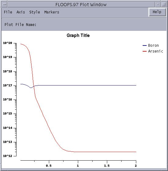
| This code section will draw the boron and arsenic concentrations at the left edge of the device. Both lines are on the same plot.
| |
| [[Image:onedblt.gif]]
| |
| | |
| === Grid Plot ===
| |
| | |
| We create a structure with an interesting grid using the commands:
| |
| | |
|
| |
| Grid2D
| |
| foreach m [mater] {Smooth $m}
| |
| | |
| This smooths each region of the mesh.
| |
| | |
|
| |
| foreach m [ [[materCommand | mater]] ] {
| |
| [[BLTplot | CreateBound]] $Win $m [ [[boundCommand | bound]] $m]
| |
| }
| |
| FlipY $Win 1
| |
| | |
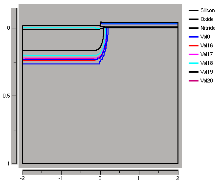
| This code section outlines each section. The grid can be plotted using a combination of the element command and the CreateLine command.
| |
| | |
| foreach m [ [[materCommand | mater]] ] {
| |
| [[BLTplot | CreateBound]] $Win $m [ [[elementCommand | element]] $m]
| |
| }
| |
| | |
| Each material has its grid added to the plot. After some [[BLTWindow | property editing]], the plot looks like:
| |
| | |
| [[Image:grid.gif]]
| |
| | |
| == XGraph Window Examples ==
| |
| | |
| === Contour and Color Plots ===
| |
| | |
| A structure is created with the following set of commands:
| |
| | |
|
| |
| Grid2D
| |
| [select.html sel] z=1.0e17 name=Boron store
| |
| sel z=1.0e15 name=Arsenic store | | sel z=1.0e15 name=Arsenic store |
| [../floops/implant.htm implant] arsenic dose=1.0e15 energy=20 | | implant arsenic dose=1.0e15 energy=20 |
| [../floops/strip.html strip] photo=az | | strip photo=az |
| [../floops/diffuse.html diffuse] time=5 temp=1100 dry | | diffuse time=5 temp=1100 dry |
|
| |
|
| <br /> The plot is created with:<br /> | | <br /> The plot is created with:<br /> |
|
| |
|
| [plot.2d.html plot.2d] bound fill | | plot.2d bound fill |
| [select.html sel] z = Boron-Arsenic | | sel z = Boron-Arsenic |
| [contour.html contour] val = 0.0 | | contour val = 0.0 |
| [select.html sel] z = log10(abs(Boron-Arsenic)) | | sel z = log10(abs(Boron-Arsenic)) |
| for {set i 15} {$i <= 20.0} {incr i} { | | for {set i 15} {$i <= 20.0} {incr i} { |
| [contour.html contour] val = $i | | contour val = $i |
| } | | } |
|
| |
|
| This code section will draw the [plot.2d.html outline] of the device and stretch it to fill the plot window. The next line [select.html selects] the doping concentration and [contour.html plot]s a line along the metallurgical junction. Then plot variable is selected to the log base 10 of the absolute doping concentration. A loop from 15 to 20 follows with [contour.html contour] lines being drawn each decade for both p- and n-type doping. The resulting plot:[[Image:cc.gif]] | | This code section will draw the outline of the device and stretch it to fill the plot window. The next line selects the doping concentration and plots a line along the metallurgical junction. Then plot variable is selected to the log base 10 of the absolute doping concentration. A loop from 15 to 20 follows with contour lines being drawn each decade for both p- and n-type doping. The resulting plot: |
| | |
| | [[Image:cc.gif]] |
|
| |
|
| === One-Dimensional Plots ===
| | = One-Dimensional Plots = |
|
| |
|
| Using the same structure as before, we can perform depth plots through several regions of the device. | | Using the same structure as before, we can perform depth plots through several regions of the device. |
|
| |
|
| | | |
| [select.html sel] z=log10(Boron) | | sel z=log10(Boron) |
| [plot.1d.html plot.1d] y=-2.0 | | plot.1d y=-2.0 |
| [select.html sel] z=log10(Arsenic) | | sel z=log10(Arsenic) |
| [plot.1d.html plot.1d] y=-2.0 !cle | | plot.1d y=-2.0 !cle |
|
| |
|
| This code section will draw the boron and arsenic concentrations at the left edge of the device. Both lines are on the same plot: [[Image:onedblt.gif]] | | This code section will draw the boron and arsenic concentrations at the left edge of the device. Both lines are on the same plot: [[Image:onedblt.gif]] |
Contour and Color Plots
A structure is created with the following set of commands:
Grid2D
sel z=1.0e17 name=Boron store
sel z=1.0e15 name=Arsenic store
implant arsenic dose=1.0e15 energy=20
strip photo=az
diffuse time=5 temp=1100 dry
The plot is created with:
plot.2d bound fill
sel z = Boron-Arsenic
contour val = 0.0
sel z = log10(abs(Boron-Arsenic))
for {set i 15} {$i <= 20.0} {incr i} {
    contour val = $i
}
This code section will draw the outline of the device and stretch it to fill the plot window. The next line selects the doping concentration and plots a line along the metallurgical junction. Then plot variable is selected to the log base 10 of the absolute doping concentration. A loop from 15 to 20 follows with contour lines being drawn each decade for both p- and n-type doping. The resulting plot:
One-Dimensional Plots
Using the same structure as before, we can perform depth plots through several regions of the device.
sel z=log10(Boron)
plot.1d y=-2.0
sel z=log10(Arsenic)
plot.1d y=-2.0 !cle
This code section will draw the boron and arsenic concentrations at the left edge of the device. Both lines are on the same plot: